Creating a Tree & States Data File

PieTree does not perform ancestral state reconstructions itself. So if node states are to be estimated and displayed, that analysis must be done elsewhere.

Here is an example of such an analysis, using the R package diversitree. The results are written to a file formatted for use by PieTree. (That file format is described here: Input tree file)

library(diversitree)
set.seed(2)

### Simulate a tree with three character states.  (See the diversitree tutorial.)

# lambda = speciation, mu = extinction, q = character state transition
# lambda1 lambda2 lambda3 mu1 mu2 mu3 q12 q13 q21 q23 q31 q32
pars <- c(0.1, 0.15, 0.2, 0.03, 0.045, 0.06, 0.05, 0, 0.05, 0.05, 0, 0.05)

phy <- tree.musse(pars, max.t = 50, x0 = 1)
states <- phy$tip.state

### Alternatively, you could read in your real data with ape commands.
### If your tree lacks node labels, use something like:
###    phy$node.label <- paste("node", seq(Nnode(phy)), sep="")

### Estimate MuSSE rates.  Note: this is an illustration, not a thorough analysis!

lik <- make.musse(phy, states, k = 3)
p <- starting.point.musse(phy, 3)
rates <- coef(find.mle(lik, p))

### Perform ancestral state reconstruction.

anc <- asr.marginal(lik, rates)
colnames(anc) <- phy$node.label

### Write the results to a .ttn file.  Note that the state numbers must start from 0.
### tree string, tip states, node state estimates

outfile <- "tree3.ttn"
write.tree(phy, file = outfile)
write.table(states-1, file = outfile, col.names = F, quote = F, append = T)
write.table(t(anc), file = outfile, col.names = F, quote = F, append = T)

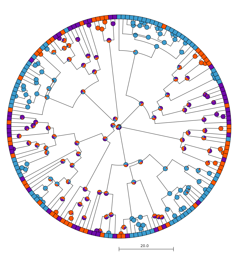
Take a look at the results:

$ PieTree --treefile tree3.ttn --shape radial --color0 "(0.44,0.04,0.67)" \
  --color1 "(1,0.34,0)" --color2 "(0.24,0.62,0.82)" --tipnamesize 0 --nodenamesize 0 \
  --scalebar 20

It’s of course possible to produce a similar image directly in R. I don’t think it looks quite as nice, however, and I find it much more frustrating to tweak things like spacing there.